Resources linked in this doc:

1. Notes on Capital vol. 3, ch. 10
2. Worksheet and applet: Extracting surplus value from workers
3. PDF: Set-theoretical notes on the value form for STEM majors
4. Slideshow: What is money? (main source: Suzanne de Brunhoff, Marx on Money)

As a working teacher, I’m always thinking about ways to make the history of ideas accessible to ordinary people—say, the average undergrad or advanced high school student. Some people publish articles. Some people tweet. I mostly make slideshows and typeset mathematical notes.

1. Notes on Capital vol. 3, ch. 10, “The equalization of the general rate of profit during competition. Market prices and market values. Surplus profit” (2024)

This document begins by presenting mathematical notation suitable for formalizing the relations between values and prices at the commodity, sectoral and global level as given in Capital vol. 3, part 2 (ch. 8-12).

The rest of the document consists of (incomplete) notes for a very close reading of chapter 10. I believe the importance of this chapter has been overlooked for 100+ years in large part due to the tragic distraction of the “transformation problem” debate, which tended to focus on chapter 9 following Bortkiewicz (1907).

I believe the relevant passages in Theories of surplus-value have also been underdiscussed in the past hundred years, although for less tendentious reasons. It’s a medium-term goal (hobby horse) of mine to show that Marx’s theory of market prices in TSV and Cap 3 can be given a consistent mathematical formulation.

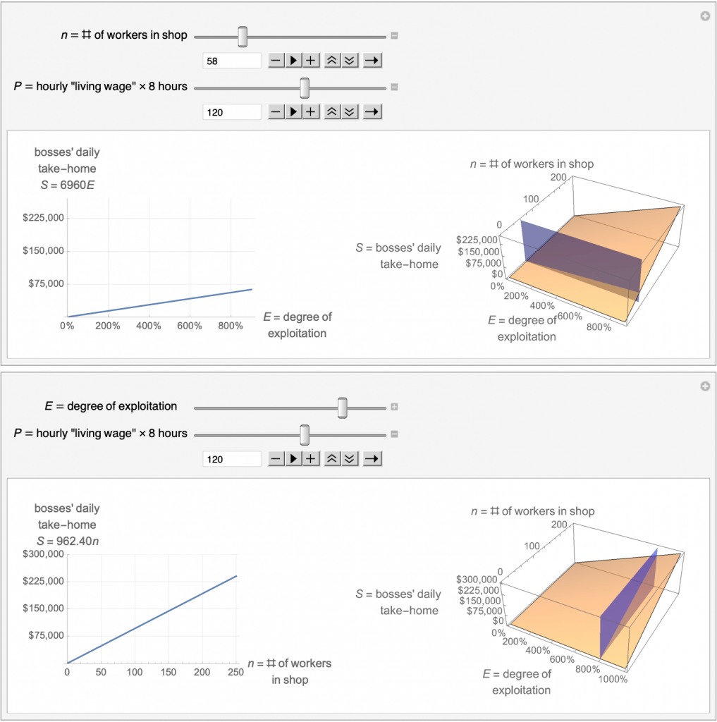
2. Worksheet: Extracting surplus value from workers (2021)

I use this handout when teaching the x and y axis to adults. It introduces Marx’s definition of the rate of exploitation as given in Capital, vol. 1, ch. 11.

We also experiment with varying the rate of exploitation, the wage and the length of the working day in the Mathematica applet pictured below.

3. Notes on the value form for STEM majors (2022)

The linked document (PDF) is an incomplete first attempt to state mathematical models of certain ideas in Capital in a way that’s accessible to math educators and advanced undergrad STEM majors with no background in economics.

In particular, the value form as given in Capital vol. 1, ch. 1 is presented in terms of elementary set theory, graph theory and linear algebra. The presentation of the value form might be used by a math instructor for an “introduction to proofs” course, e.g. when covering equivalence relations “modding out”.

There’s more work that’s not in the document (e.g. the model behind the applet pictured above). Without it, some of my formal choices (like calling “commodity” a random variable) may seem odd [the notes on Cap 3 ch 10 clarify these formal choices]. I’ve spotted some errors in the later (and most incomplete) sections, too. This project lives on my back-burner and will be completed in n ≥ 2 years, where n is unknown.

3. Marx on money (2023)

This slideshow presents key points in Suzanne de Brunhoff’s interpretation of Marx’s theory of money. My main source was her 1976 book, Marx on money.

4. Notes on the genealogy of Marxian political economy (2023)

Extremely unfinished notes (in slideshow format) on points of agreement and disagreement between Marx and classical political economists including James Steuart, the Physiocrats, Adam Smith, and (least finished of all) Ricardo.

The slideshow includes teaser slides for “heterodox economics” and the “transformation problem” meant to inspire interest in these topics.